cubble: An R Package for Organizing and Wrangling Multivariate Spatio-temporal Data
H. Sherry Zhang
Joint work with Dianne Cook, Patricia Menéndez, Ursula Laa, and Nicolas Langrené
https://sherryzhang-user2022.netlify.app
2022-06
Spatial data
stations_sfSimple feature collection with 59 features and 6 fieldsGeometry type: POINTDimension: XYBounding box: xmin: 141.2652 ymin: -39.1297 xmax: 153.3633 ymax: -28.9786Geodetic CRS: GDA94# A tibble: 59 × 7 id long lat elev name wmo_id <chr> <dbl> <dbl> <dbl> <chr> <dbl>1 ASN00047016 141. -34.0 43 lake victo… 946922 ASN00047019 142. -32.4 61 menindee p… 946943 ASN00048015 147. -30.0 115 brewarrina… 955124 ASN00048027 146. -31.5 260 cobar mo 947115 ASN00048031 149. -29.5 145 collareneb… 95520# … with 54 more rows, and 1 more variable:# geometry <POINT [°]>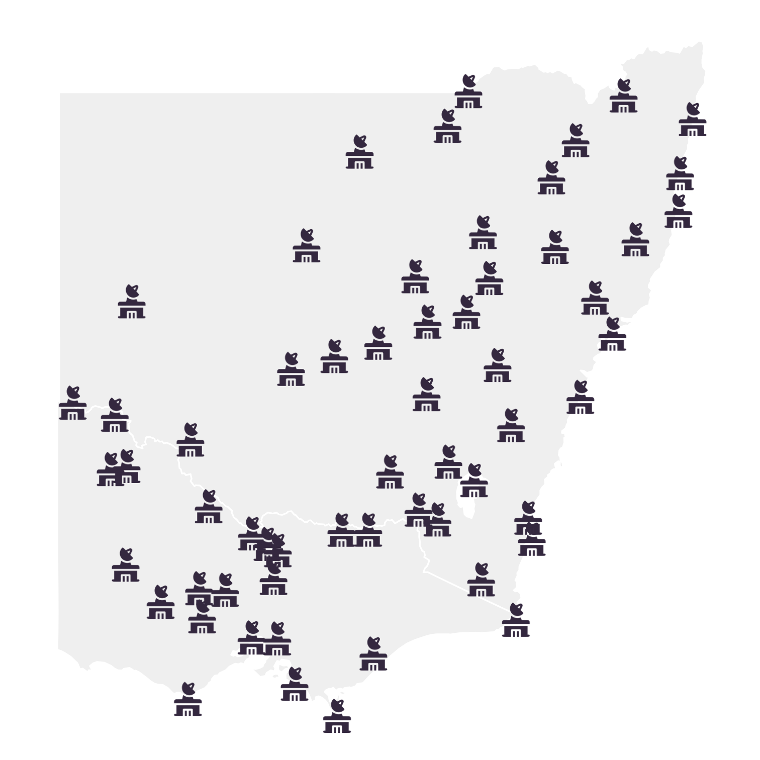
Thanks everyone for coming
The title of my talk today is
Here is the link to this slide and the link now is also available in the chat.
Spatial data is a common type of data and here there are 59 weather stations distributed in New South Wales and Victoria in Australia
The data is organised in an
sfclass and the packagesfprovides various geometrical operations in the space for this class
Temporal data
ts# A tsibble: 1,099,052 x 3 [1D]# Key: id [59] id date tmax <chr> <date> <dbl>1 ASN00047016 1971-01-01 25 2 ASN00047016 1971-01-02 26.93 ASN00047016 1971-01-03 27.54 ASN00047016 1971-01-04 30 5 ASN00047016 1971-01-05 34.4# … with 1,099,047 more rows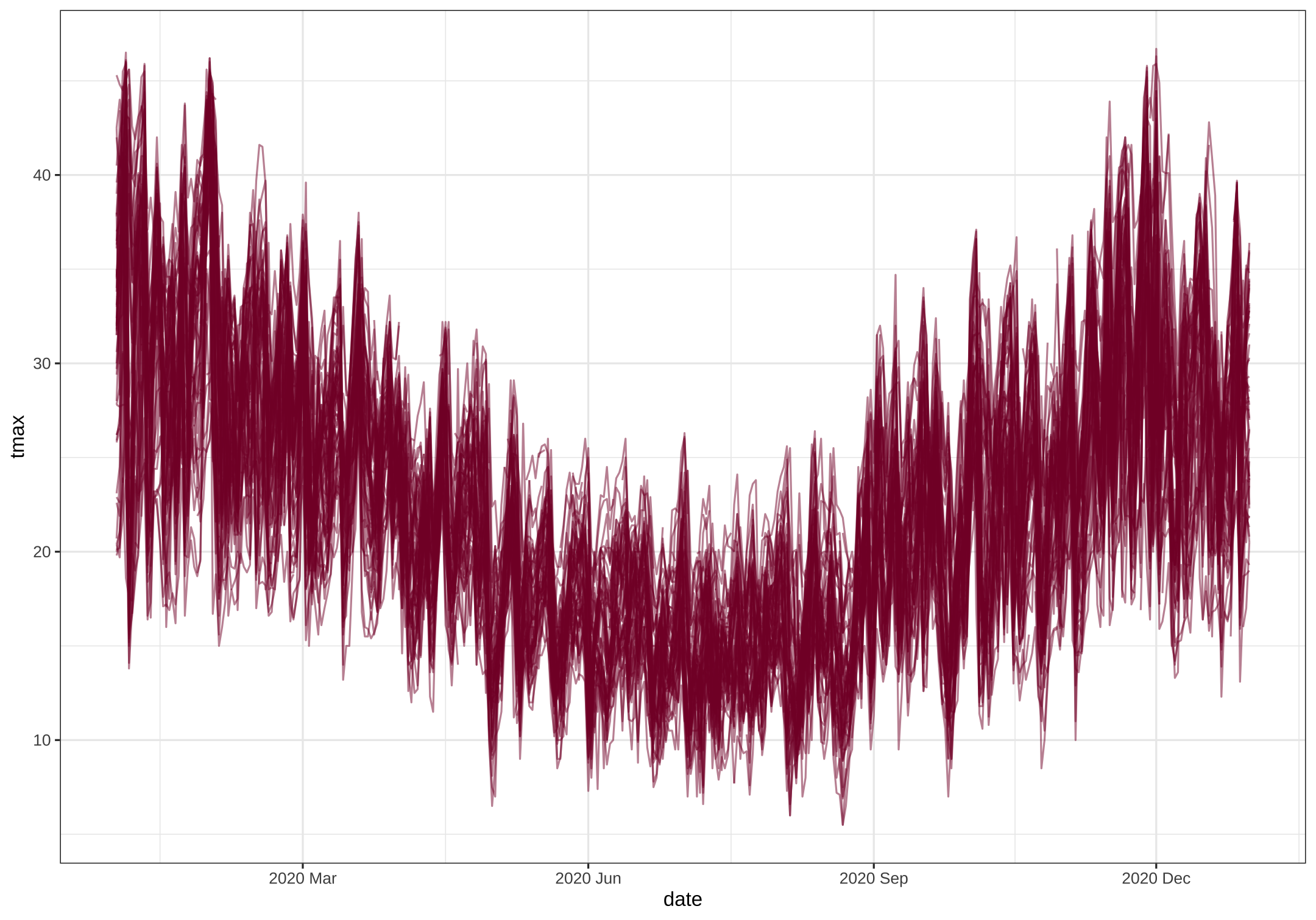
Temporal data is another common data type
Here I'm showing you some daily historical temperature data for those 59 stations.
On the right, a fraction of the data in year 2020 is plotted
This data is stored in a
tsibbleclass, withidas the key to define each series anddateas the index to define the time stamp.The
tsibbleclass allows you to wrangle temporal data and build temporal models.
Spatio-temporal data
When left joining an sf object with a tsibble object, the tsibble class (tbl_ts) gets lost:
out <- stations_sf %>% left_join(ts, by = "id")class(out)[1] "sf" "tbl_df" "tbl" "data.frame"When left joining the other way around, you lost the sf class:
out2 <- ts %>% left_join(stations_sf, by = "id")class(out2)[1] "tbl_ts" "tbl_df" "tbl" "data.frame"However, spatial objects and temporal objects do not naturally work well together for spatio-temporal analysis.
Here let me give you some examples
If I join an sf object with a tsibble object, the tsibble class would gets lost
If we join the data the other way around, the
sfclass will get lost.
Multivariate spatio-temporal data
You can manually enforce the joined object to have both classes:
out2 <- ts %>% left_join(stations_sf, by = "id")out3 <- out2 %>% st_as_sf()class(out3)[1] "sf" "tbl_ts" "tbl_df" "tbl" "data.frame"but the class lost again after a tsibble operation:
out4 <- out3 %>% tsibble::fill_gaps()class(out4)[1] "tbl_ts" "tbl_df" "tbl" "data.frame"We can manually enforce the joined object to have both classes with the function
st_as_sf()But the class label can still get lost during operations.
Here I use a tsibble function
fill_gapsand the result doesn't have thesfclassAlso, taking a step back, the left join approach on spatial and temporal data is not necessarily the best way to structure spatio-temporal data
This is because all the feature geometries are repeated multiple times, especially for long daily data, like the temporal data I just show you.
This motivates a new data representation
Cubble
A new tidy data structure to organise and wrangle spatio-temporal data
Today I will introduce a new data structure, called cubble, to organise spatio-temporal data.
And we will see how data wangling with cubble can be fun
Multivariate spatio-temporal cubes
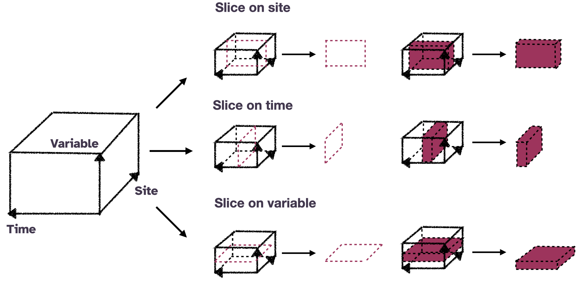
Conceptually spatio-temporal data can be thought of as a data cube
In this cube, the three axes are Time, Site, and Variable.
The axis Site defines the location of the entities
The axis Variable is used to represent multivariate information.
We define our data cube slightly different from a conventional cube to avoid introducing hypercubes for multivariate information.
Operations on multivariate spatio-temporal data can be thought of as slicing and dicing on the cube.
Although The data cube is conceptually convenient, for data wrangling, a 3D array structure may not sufficiently rich, for example, to wrangle special date time classes.
Cubble basics
Now I will demonstrate how cubble organises spatio-temporal data with two forms.
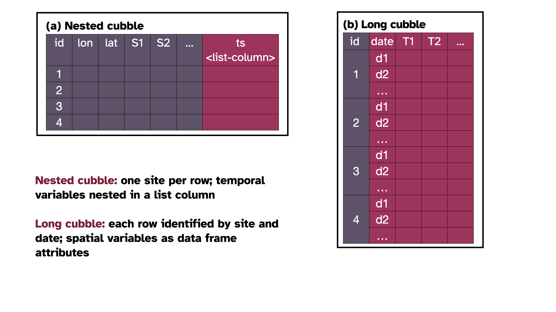
The nested form organises each site in a row.
Spatial variables fixed for each site can be directly wrangled.
Temporal variables varied across time are nested in a list column called
ts.
On the other hand, the long form cubble organises each row by a combination of site and date, similar to a
tsibble.Temporal variables can be directly wrangled and
spatial variables are stored as a data attribute, which I will show you shortly in the code.
Switching focus between time and space
In a spatio-temporal analysis, we may want to first subset a few location and then explore their temporal patterns.
We may also want to first calculate some temporal features and then investigate its spatial distribution.
These analyses would require switch between the nested form and the long form in a cubble
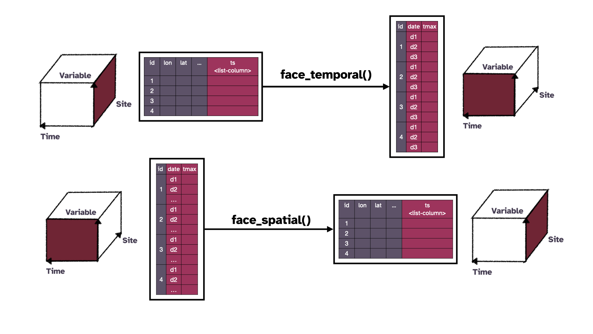
The function
face_temporal()turns a nested cubble into the long form andThis can be used to first filter the location on the nested form and then use
face_temporal()to switch the data into the long form and then make temporal summariesThe inverse of
face_temporal()isface_spatial(), which switches the long cubble into a nested oneWith
face_spatial()we can first make some calculations on the temporal side and switch back to the nested form to view its spatial distribution on the map
Creating a cubble
weather <- as_cubble(list(spatial = stations_sf, temporal = ts), key = id, index = date, coords = c(long, lat))Now I'm going to show you how to create a cubble from the two data we have
Here you specify the two separate objects in a list with the name
spatialandtemporal.Then you can specify the
keyand theindexas what you would do when creating atsibble.The
coordsargument needs to be specified in the order of longitude and latitude.
Creating a cubble
weather <- as_cubble(list(spatial = stations_sf, temporal = ts), key = id, index = date, coords = c(long, lat))# cubble: id [59]: nested form [sf]# bbox: [141.26, -39.13, 153.37, -28.97]# temporal: date [date], tmax [dbl] id long lat elev name wmo_id geometry ts <chr> <dbl> <dbl> <dbl> <chr> <dbl> <POINT [°]> <list> 1 ASN00047016 141. -34.0 43 lake victoria storage 94692 (141.2652 -34.0398) <tbl_ts>2 ASN00047019 142. -32.4 61 menindee post office 94694 (142.4173 -32.3937) <tbl_ts>3 ASN00048015 147. -30.0 115 brewarrina hospital 95512 (146.8651 -29.9614) <tbl_ts>4 ASN00048027 146. -31.5 260 cobar mo 94711 (145.8294 -31.484) <tbl_ts>5 ASN00048031 149. -29.5 145 collarenebri (albert st) 95520 (148.5818 -29.5407) <tbl_ts># … with 54 more rowsNow I'm going to show you how to create a cubble from the two data we have
Here you specify the two separate objects in a list with the name
spatialandtemporal.Then you can specify the
keyand theindexas what you would do when creating atsibble.The
coordsargument needs to be specified in the order of longitude and latitude.
- This creates a cubble in the nested form.
Creating a cubble
weather <- as_cubble(list(spatial = stations_sf, temporal = ts), key = id, index = date, coords = c(long, lat))# cubble: id [59]: nested form [sf]# bbox: [141.26, -39.13, 153.37, -28.97]# temporal: date [date], tmax [dbl] id long lat elev name wmo_id geometry ts <chr> <dbl> <dbl> <dbl> <chr> <dbl> <POINT [°]> <list> 1 ASN00047016 141. -34.0 43 lake victoria storage 94692 (141.2652 -34.0398) <tbl_ts>2 ASN00047019 142. -32.4 61 menindee post office 94694 (142.4173 -32.3937) <tbl_ts>3 ASN00048015 147. -30.0 115 brewarrina hospital 95512 (146.8651 -29.9614) <tbl_ts>4 ASN00048027 146. -31.5 260 cobar mo 94711 (145.8294 -31.484) <tbl_ts>5 ASN00048031 149. -29.5 145 collarenebri (albert st) 95520 (148.5818 -29.5407) <tbl_ts># … with 54 more rows- 59 stations, in the nested form, and is a subclass of
sf - The available temporal variables are
dateandtmax - Also, each temporal component in the list column is a tsibble (
tbl_ts)
Now I'm going to show you how to create a cubble from the two data we have
Here you specify the two separate objects in a list with the name
spatialandtemporal.Then you can specify the
keyand theindexas what you would do when creating atsibble.The
coordsargument needs to be specified in the order of longitude and latitude.
- This creates a cubble in the nested form.
- The header of a cubble tells you that this data has
Cubble summary (1/2)
weather_long <- weather %>% face_temporal()
weather_long
# cubble: date, id [59]: long form [tsibble]# bbox: [141.26, -39.13, 153.37, -28.97]# spatial: long [dbl], lat [dbl], elev [dbl],# name [chr], wmo_id [dbl], geometry [POINT# [°]] id date tmax <chr> <date> <dbl>1 ASN00047016 1971-01-01 25 2 ASN00047016 1971-01-02 26.93 ASN00047016 1971-01-03 27.54 ASN00047016 1971-01-04 30 5 ASN00047016 1971-01-05 34.4# … with 1,099,047 more rows- a long form cubble as the subclass of
tsibble - the third row now shows the spatial variables
We can pivot this object into the long form with
face_temporal()Now the object
weather_longis a long form cubble and it is a subclass of tsibbleThe third line in the header now changes to see the available spatial variables
Cubble summary (1/2)
weather_long <- weather %>% face_temporal()
weather_long
# cubble: date, id [59]: long form [tsibble]# bbox: [141.26, -39.13, 153.37, -28.97]# spatial: long [dbl], lat [dbl], elev [dbl],# name [chr], wmo_id [dbl], geometry [POINT# [°]] id date tmax <chr> <date> <dbl>1 ASN00047016 1971-01-01 25 2 ASN00047016 1971-01-02 26.93 ASN00047016 1971-01-03 27.54 ASN00047016 1971-01-04 30 5 ASN00047016 1971-01-05 34.4# … with 1,099,047 more rows- a long form cubble as the subclass of
tsibble - the third row now shows the spatial variables
attr(weather_long, "spatial")Simple feature collection with 59 features and 6 fieldsGeometry type: POINTDimension: XYBounding box: xmin: 141.2652 ymin: -39.1297 xmax: 153.3633 ymax: -28.9786Geodetic CRS: GDA94# A tibble: 59 × 7# Rowwise: id id long lat elev name wmo_id <chr> <dbl> <dbl> <dbl> <chr> <dbl>1 ASN00047016 141. -34.0 43 lake victo… 946922 ASN00047019 142. -32.4 61 menindee p… 946943 ASN00048015 147. -30.0 115 brewarrina… 955124 ASN00048027 146. -31.5 260 cobar mo 947115 ASN00048031 149. -29.5 145 collareneb… 95520# … with 54 more rows, and 1 more variable:# geometry <POINT [°]>We can pivot this object into the long form with
face_temporal()Now the object
weather_longis a long form cubble and it is a subclass of tsibbleThe third line in the header now changes to see the available spatial variables
The spatial variables are stored in the
spatialattribute, which you can see through this command.Here it is stored as an sf object
Cubble summary (2/2)
weather_back <- weather_long %>% face_spatial()
weather_back
# cubble: id [59]: nested form [sf]# bbox: [141.26, -39.13, 153.37, -28.97]# temporal: date [date], tmax [dbl] id long lat elev name wmo_id geometry ts <chr> <dbl> <dbl> <dbl> <chr> <dbl> <POINT [°]> <list> 1 ASN00047016 141. -34.0 43 lake victoria storage 94692 (141.2652 -34.0398) <tbl_ts>2 ASN00047019 142. -32.4 61 menindee post office 94694 (142.4173 -32.3937) <tbl_ts>3 ASN00048015 147. -30.0 115 brewarrina hospital 95512 (146.8651 -29.9614) <tbl_ts>4 ASN00048027 146. -31.5 260 cobar mo 94711 (145.8294 -31.484) <tbl_ts>5 ASN00048031 149. -29.5 145 collarenebri (albert st) 95520 (148.5818 -29.5407) <tbl_ts># … with 54 more rowsidentical(weather_back, weather)
[1] TRUEHere is the code example of using the function
face_spatial()on the long form cubbleThis would give us the nested cubble before making the switch to the long form
Pipeline with cubble
cb_obj %>%
  {{ Your spatial analysis }} %>%
  face_temporal() %>%
  {{ Your temporal analysis }} %>%
  face_spatial() %>%
  {{ Your spatial analysis }}
spatial <- stations_sf %>%
  {{ Your spatial analysis }}

##############################
# more subsetting step if temporal analysis
# depends on spatial results
sp_id <- spatial %>% pull(id)
ts_subset <- ts %>% filter(id %in% sp_id)
##############################

temporal <- ts_subset %>%
  {{ Your temporal analysis }}

##############################
# more subsetting step if spatial analysis
# depends on temporal results
ts_id <- temporal %>% pull(id)
sp_subset <- spatial %>% filter(id %in% ts_id)
##############################

sp_subset %>%
  {{ Your spatial analysis }}
Here is a syntax comparison with and without cubble
With cubble, you can do some spatial analysis in the nested form, pivot it to the long form for some temporal analysis, and then pivot it back to the nested form for some additional spatial analysis.
Sometimes, the spatial analysis include extracting some interesting sites.
Without cubble, you will need to first pull out those interesting ids, and then filter the temporal data on these sites.
Similar steps can also happen in the temporal analysis and the spatial data needs to be updated.
In cubble, these updates are automatically handled by
face_temporal()andface_spatial()and no manual updates are needed.Also the cubble pipeline chains all the operations together with no intermediate objects created in the workflow.
Spatio-temporal analysis in cubble
A glyph map example
Some analysis uses both spatial and temporal of variables at the same time.
An example of this is making glyph maps.
Here I will first show you a toy example before rolling out to the full picture
Transform a dot into a glyph
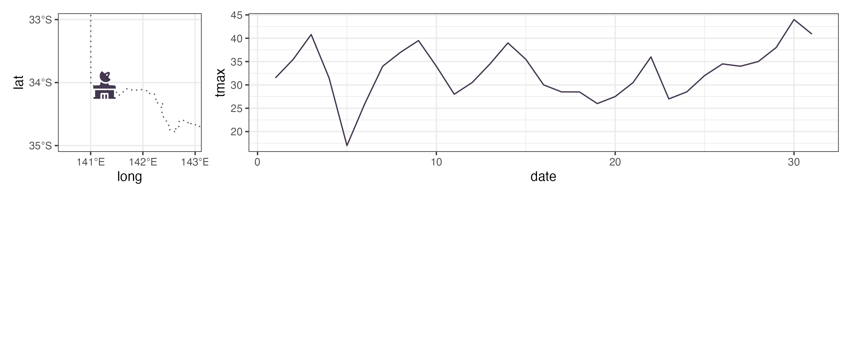
A glyph map is a transformation of temporal coordinates into the spatial coordinates, so that temporal information can be visualised on the map.
Here I have one weather station on the map and its maximum temperature on each day in January 2020
Transform a dot into a glyph
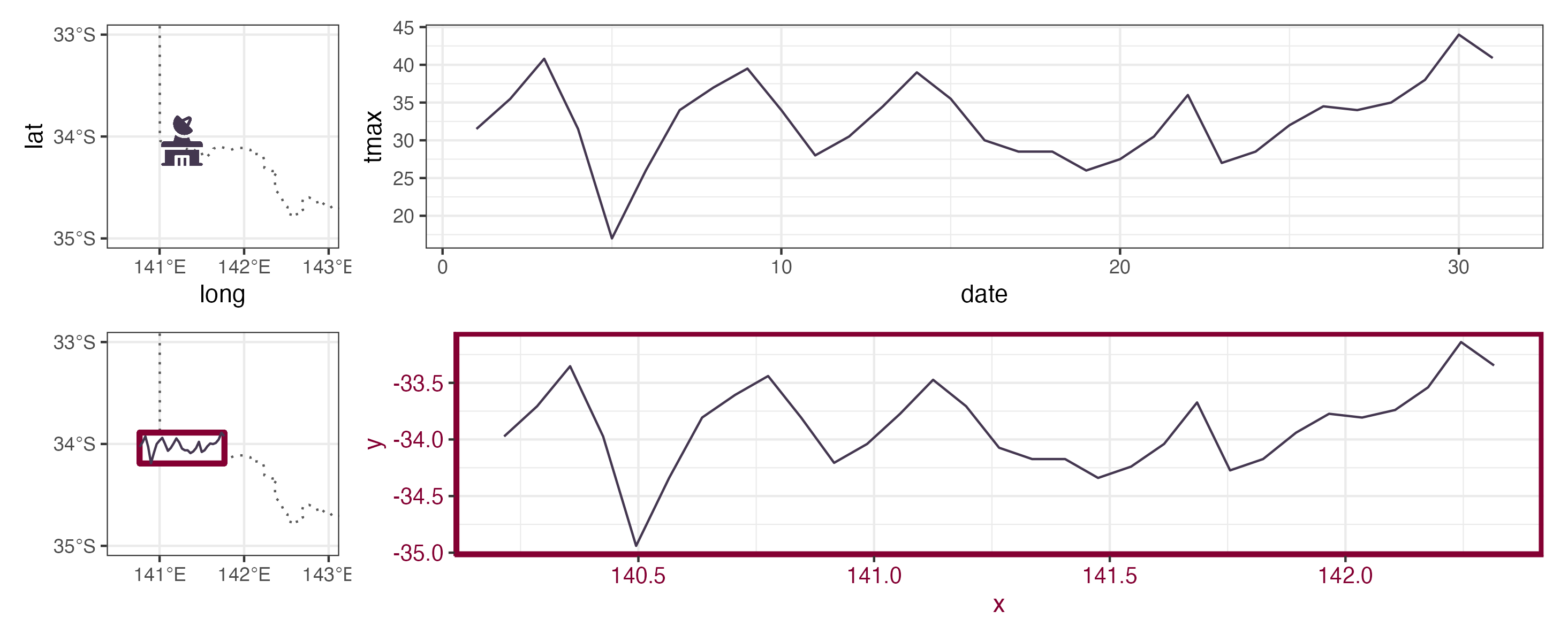
A glyph map uses linear algebra to make this transformation
You can see here the line in the bottom right plot does not change but its coordinates have been changed to the spatial coordinates
In a glyph map, the spatial coordinates are called the major coordinates and the temporal coordinates are the minor coordinates.
In the word of ggplot, we need four aesthetics to make a glyph map. Here they are longitude, latitude, date, and tmax.
Transformation to glyphmap
cb_glyph <- weather_long %>% unfold(long, lat)
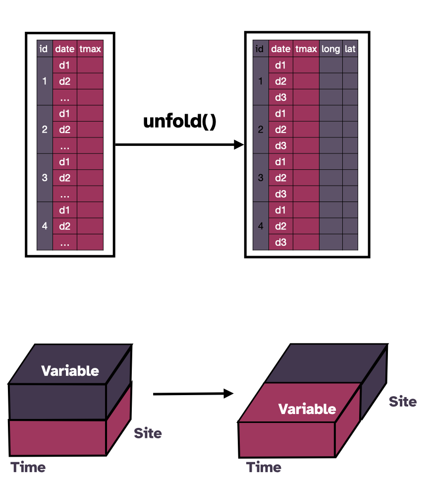
# cubble: date, id [59]: long form [tsibble]# bbox: [141.26, -39.13, 153.37, -28.97]# spatial: long [dbl], lat [dbl], elev [dbl], name [chr],# wmo_id [dbl], geometry [POINT [°]] id date tmax long lat <chr> <date> <dbl> <dbl> <dbl>1 ASN00047016 1971-01-01 25 141. -34.02 ASN00047016 1971-01-02 26.9 141. -34.03 ASN00047016 1971-01-03 27.5 141. -34.04 ASN00047016 1971-01-04 30 141. -34.05 ASN00047016 1971-01-05 34.4 141. -34.0# … with 1,099,047 more rowscb_glyph %>% ggplot(aes(x_major = long, y_major = lat, x_minor = date, y_minor = tmax)) + geom_glyph()To work with ggplot2, all the four variables need to be in the same table.
In cubble you can use the function
unfold()to relocate spatial variables into the long form.Here I have the diagram, cube, and the code to demonstrate this function.
This is how the data looks like after the unfold
After this, the data can be piped into the ggplot with the four aesthetics need for
geom_glyph()to draw the glyph map.
Example: Australian temperature comparison
Now here is an full example that combines everything I have introduced in this talk, to analyse historical temperature data in Australia.
We have maximum temperature dated back to the 70s, which allows us to compare the maximum temperature between now and then, and also across space.
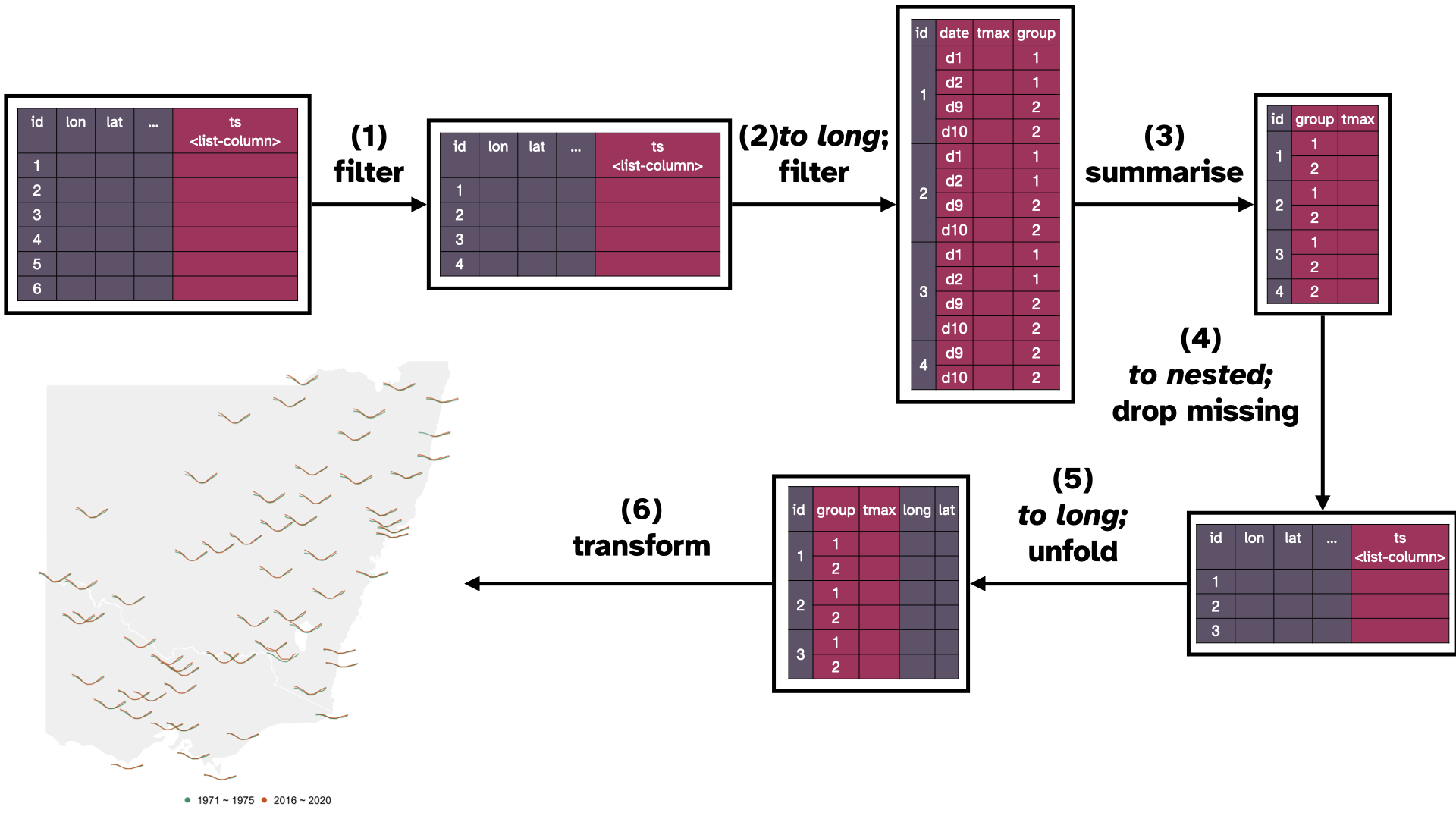
The diagram here shows each step needed in this analysis
The data I have shown you in this talk is a subset from all the weather stations in Australia and there are hundreds of them.
The first step here is to narrow it down to those in New South Wales and Victoria
Then we pivot it into the long form to select a historical segment (from 1971 - 1975) and a recent segment (from 2016 to 2020) in step 2.
In step 3, still in the long form, maximum temperature is summarised into monthly average in each period
A quick check on the number of observations reveals that some stations don't have temperature recorded at both groups - look at id 4
We remove them in the nested form in step 4
In step 5 and 6 we unfold longitude and latitude with temporal variables and make the glyph map with
geom_glyph()
Example: Australian temperature comparison
tmax <- DATA %>%
  {{filter NSW & VIC stations}} %>%
  face_temporal() %>%
  {{group by month and period (71-75, 16-20)}} %>%
  {{summarise into monthly average}} %>%
  face_spatial() %>%
  {{filter out sites with no historical record}} %>%
  face_temporal() %>%
  unfold(long, lat)

tmax %>%
  ggplot(aes(x_minor = month, y_minor = tmax,
             x_major = long, y_major = lat)) +
  geom_glyph() +
  ...
This is the code version of the diagram illustration
Functions highlighted in light yellow are developed in the cubble package
Spatial operations are highlighted in purple and temporal ones in pink
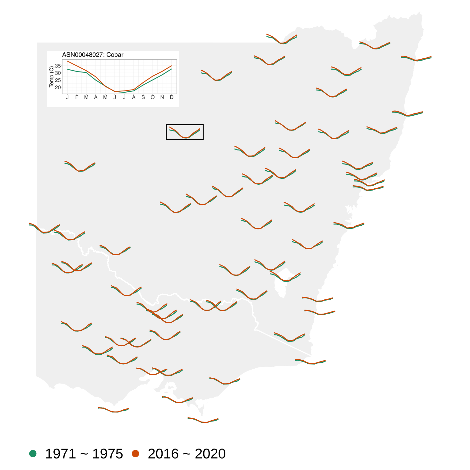
On the top left of the plot is a more annotated version of the glyph for one specific station Cobar.
Australia has a U-shape temperature curve and if you look carefully, the inland NSW stations has a noticeable higher average maximum temperature in January in recent years.
More you can do with cubble
- Pick up unmatched entries from the spatial and temporal inputs
There are more things cubble can do
More you can do with cubble
Pick up unmatched entries from the spatial and temporal inputs
Merge two data sources by spatial and temporal similarities
There are more things cubble can do
More you can do with cubble
Pick up unmatched entries from the spatial and temporal inputs
Merge two data sources by spatial and temporal similarities
Handle (spatial) hierarchical structure of sites
There are more things cubble can do
More you can do with cubble
Pick up unmatched entries from the spatial and temporal inputs
Merge two data sources by spatial and temporal similarities
Handle (spatial) hierarchical structure of sites
Input data can be of various forms, including a single combined data frame and netCDF
There are more things cubble can do
Additional Information
Slides created via the R package xaringan and xaringanthemer, available at
https://sherryzhang-user2022.netlify.app
Install the latest version of cubble:
remotes::install_github("huizezhang-sherry/cubble")
Collaborators: Dianne Cook, Patricia Menéndez, Ursula Laa, and Nicolas Langrené
This wraps up my presentation today
Cubble has already made its way to CRAN
There has been some major changes made in the last few months and we plan to make an CRAN update very soon.
So keep an eye on my github and twitter.
Thanks for your time :)